Stress Mohr Circle

Classical Description

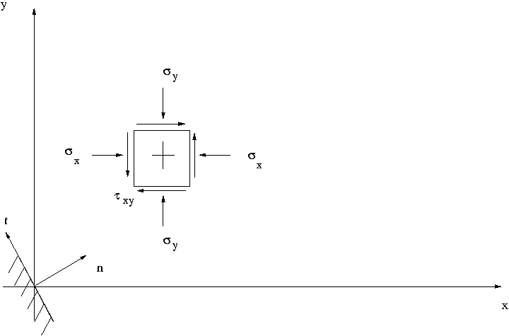
Classical description can be found HERE. Figure show the convention of negative value for shear positive in the x surface of the elemental cube

Vector Rotation

The global reference system components of the tension on a plane whose normal is represented by the vector

$$\left( \begin{array}{c} cos(\theta) \\ sin(\theta) \end{array} \right)$$

can be expressed by

$$\left( \begin{array}{c} p_x \\ p_y \end{array} \right)$$

and it is determined by the following inner product

$$\left( \begin{array}{c} p_x \\ p_y \end{array} \right) = \left( \begin{array}{cc} \sigma_x & \tau_{xy} \\ \tau_{xy} & \sigma_y \end{array} \right) \cdot \left( \begin{array}{c} cos(\theta) \\ sin(\theta) \end{array} \right)$$

The classical Mohr-Coulomb limit yelding law for cohesive-friction material assign a relationship between the normal and tangential components of the streeses. The previous relation has to be projected to the on the n-t plane

Using trigonometric identity

$$\sigma_n = \left( p_x \quad{,}\quad p_y \right) \cdot \left( \begin{array}{c} cos(\theta) \\ sin(\theta) \end{array} \right)$$

$$\tau_n = \left( p_x \quad{,}\quad p_y \right) \cdot \left( \begin{array}{c} -sin(\theta) \\ cos(\theta) \end{array} \right)$$

expanding

$$\sigma_n = \sigma_y + \frac{(\sigma_x-\sigma_y)}{2} + \frac{(\sigma_x-\sigma_y)}{2} cos(2 \theta) + \tau_{xy} sin(2 \theta)$$

$$\tau_{nt} = \frac{(\sigma_x-\sigma_y)}{2} sin(2 \theta) + \tau_{xy} cos(2 \theta)$$

After recognizing the mean tension:

$$\sigma_m = \sigma_y + \frac{(\sigma_x-\sigma_y)}{2}$$

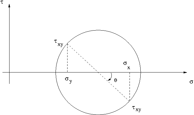
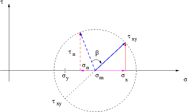
one can consider the vector from the mean pressure to the point representative of stress \( \left( \sigma_x \quad{,}\quad \tau_{xy} \right) \) with component (blue vector in the following figure):

$$\left( \begin{array}{c} \sigma_0 \\ \tau_0 \end{array} \right) $$

hence follow

$$\left( \begin{array}{c} \sigma_x \\ \tau_{xy} \end{array} \right) = \left( \begin{array}{c} \sigma_m \\ 0 \end{array} \right) + \left( \begin{array}{c} \sigma_0 \\ \tau_0 \end{array} \right)$$

$$\left( \begin{array}{c} \sigma_0 \\ \tau_0 \end{array} \right) = \left( \begin{array}{c} \sigma_x - \sigma_m \\ \tau_{xy} \end{array} \right)$$

Then the vector representing the stress on the surface of normal " n " rotated of an angle \(\theta\) respect to the "x" axis with tail at the mean pressure point, represented by the point \( \left( \sigma_n \,, \tau_n \right) \) in the stress plane, is represented by the vector rotated of \( \beta \) degrees respect to the vector \( \left( \sigma_0 \,, \tau_0 \right) \) :

the angle \( \beta \) results

$$\beta=2\theta$$

Finally

$$\left( \begin{array}{c} \sigma_{\theta} \\ \tau_{\theta} \end{array} \right) = \left( \begin{array}{cc} cos(2\theta) & sin(2 \theta) \\ -sin(2\theta) & cos(2 \theta) \end{array} \right) \cdot \left( \begin{array}{c} \sigma_0 \\ \tau_0 \end{array} \right)$$

the above vector equation represents the rotation (negative) transformation of the vector at the right hand member where \( \sigma_{\theta} \) and \( \tau_{\theta} \) are the components of the dotted vector.

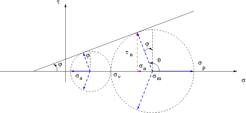
Limit Plastic State

considering the standard state of stress of a point in the soil mass
the vector representing the palstic state is obtained rotating the vector "0" till the tangent point between the circle and the limit line

the plane experiencing the limit state of stress can be obtained rotating the passive state of stress of
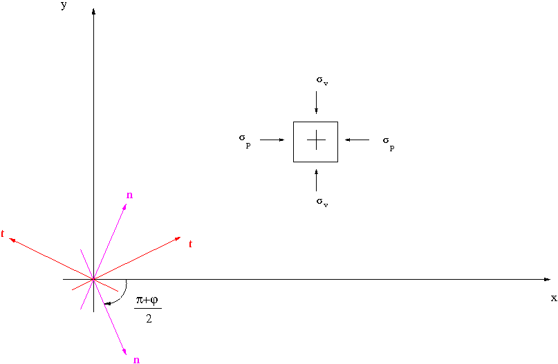$$-\frac{\frac{\pi}{2}+\phi}{2}$$
or the active state of stress of
$$\frac{\frac{\pi}{2}-\phi}{2}$$

-- RobertoBernetti - 01 Jul 2011